Understanding Term-based Retrieval methods in Information Retrieval
This article explains the intuition behinds most common term-based retrieval methods such as BM25, TF-IDF, Query Likelihood Model.
What is Information Retrieval?
The meaning of the term information retrieval (IR) can be very broad. For instance, getting your ID out of your pocket so that you can type that in a document is a simple form of information retrieval. While there are several definitions of IR, many agree that IR is about technology to connect people to information. This includes search engines, recommender systems, and dialogue systems etc. From an academic perspective, information retrieval might be defined as:
Information retrieval (IR) is finding material (usually documents) of an unstructured nature (usually text) that satisfies an information need from within large collections (usually stored on computers).
Manning et al., “Introduction to Information Retrieval”
Term-based Retrieval Methods
Term based retrieval methods are mathematical frameworks to defining query-document matching based on exact syntactic matching between a document and a query to estimate the relevance of documents to a given search query. The idea is that a pair of document and search query are represented by terms they contain. This article explains the intuition behinds most common term-based retrieval methods such as BM25, TF-IDF, Query Likelihood Model.
1. TF-IDF
TF-IDF deals with information retrieval problem based on Bag of Words (BOW) model, which is probably the simplest IR model. TF-IDF contains two parts: TF (Term frequency) and IDF (Inverse Document Frequency).
TF — Term Frequency
Term frequency, as the name suggests, is the frequency of term t in document d . The idea is that we assign a weight to each term in a document depending on the number of occurrences of that term in the document. The score of the document is hence equal to the term frequency, that is intended to reflect how important a word is to the document.
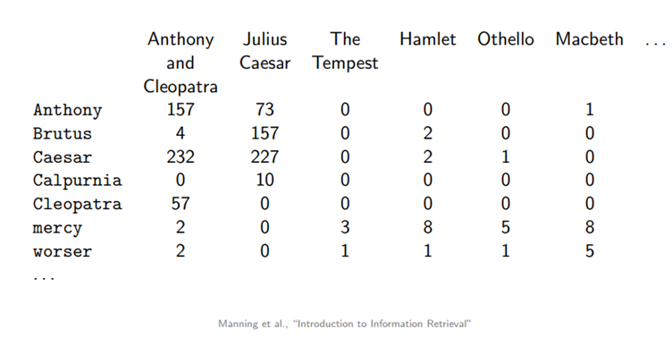
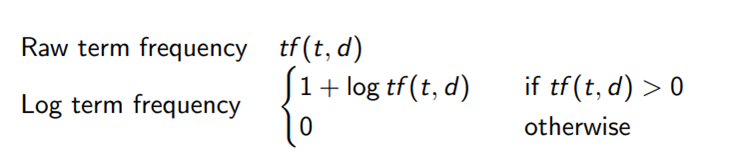
In the literature we find two commonly used formulas for term frequency, the raw term frequency that counts how often a term t appears inside a document d, and the log term frequency given by the formula below. The log has a dampening effect on larger values of term frequencies. If we look at the table above for the term ”Anthony”, it appears twice as often in Anthony and Cleopatra than in Julius Caesar. With a raw term frequency, this would imply that Anthony and Cleopatra is twice as relevant than Julius Caesar.
IDF — Inverse document frequency
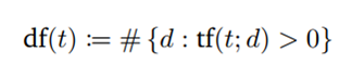
Term frequency suffers from a critical problem: All terms are considered equally important when it comes to assessing the document relevance on a query, although this is not always the case. In fact, certain terms have little or no discriminating power in determining relevance (e.g “the” may appear a whole lot in one document but contribute nothing to the relevance). To this end, we introduce a mechanism to reduce the effect of terms that occur too often in the collection to be meaningful for determining the relevance. To identify only the important terms, we can report document frequency (DF) of that term, which is the number of documents in which the term occurs. It says something about the uniqueness of the terms in the collection. The smaller DF, the more uniqueness of the given terms.
So, we are doing better. But what is the problem with DF? DF alone unfortunately tells us nothing. For instance, if DF of the term “computer” is 100, is that a rare or common term? We simply don’t know. That’s why DF needs to be put in a context, which is the size of the corpus/collection. If the corpus contains 100 documents, then the term is very common, if it contains 1M documents, the term is rare. So, let’s add the size of corpus, called N and divide to document frequency of the term.
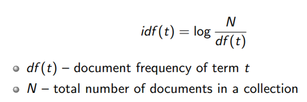
Sounds good right? But let’s say the corpus size is 1000 and the number of documents that contain the term is 1, then N/DF will be 1000. If the number of documents that contain the term is 2, then N/DF will be 500. Obviously, a small change in DF can have a very big impact on N/DF and IDF Score. It is important to keep in mind that we mainly care when DF is in a low range compared to corpus size. This is because if DF is very big, the term is common in all documents and probably not very relevant to a specific topic. In this case, we want to smooth out the change of N/DF and one simple way to do this is to take the log of N/DF. Plus, applying a log can be helpful to balance the impact of both TF and N/DF on final score. As such, if the term appears in all documents of the collection, DF will be equal to N. Log(N/DF) = log1 = 0, meaning that the term does not have any power in determining the relevance.
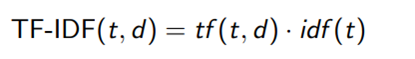
Together, we can define TF-IDF score as follows:
2. BM25
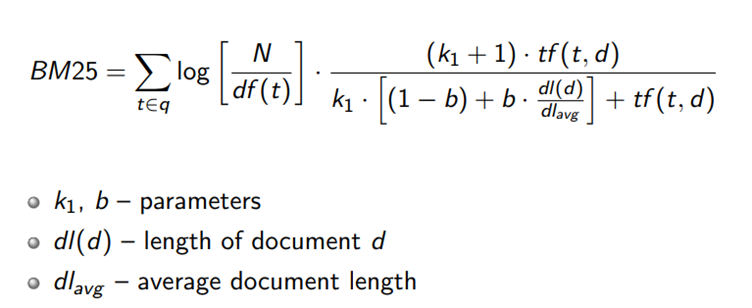
BM25 is a probabilistic retrieval framework that extends the idea of TF-IDF and improves some drawbacks of TF-IDF which concern with term saturation and document length. The full BM25 formula looks a bit scary but you might have noticed that IDF is a part of BM25 formula. Let’s break down the remaining part into smaller components to see why it makes sense.
Term Saturation and diminishing return
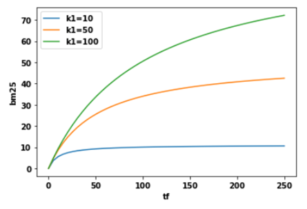
If a document contains 100 occurrences of the term “computer,” is it really twice as relevant as a document that contains 50 occurrences? We could argue that if the term “computer” occurs a large enough number of times, the document is almost certainly relevant, and any more occurrences doesn’t increase the likelihood of relevance. So, we want to control the contribution of TF when a term is likely to be saturated. BM25 solves this issue by introducing a parameter k1 that controls the shape of this saturation curve. This allows us to experiment with different values of k1 and see which value works best.
Instead of using TF, we will be using the following: (k1+1)* TF / (TF + k1)
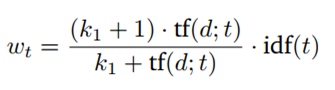
So, what does this do for us? It says that if k1 = 0, then (k1+1)*TF/TF+ k1 = 1. In this case, BM25 now turns out to be IDF. If k goes to infinity, BM25 will be the same as TF-IDF. Parameter k1 can be tuned in a way that i**_f the TF increases, at some point, the BM25 score will be saturated_** as can be seen in the figure below, meaning that the increase in TF no longer contributes much to the score.
Document Length Normalization
Another problem that is skipped in TF-IDF is document length. If a document happens to be very short and it contains “computer” once, that might already be a good indicator of relevance. But if the document is really long and the term “computer” only appears once, it is likely that the document is not about computers. We want to give a reward to term matches to short documents and penalize the long ones. However, you do not want to over-penalize because sometimes a document is long because it contains lots of contains relevant information rather than just having lots of words. So, how can we achieve this? We will introduce another parameter b, which is used to construct the normalizer: (1-b) +b*dl/dlavg in the BM25 formula. The value of parameter b must be between 0 and 1 to make it work. Now BM25 score will be the following:
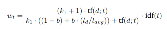
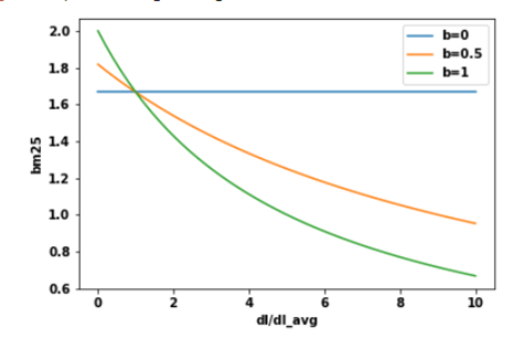
First, let us understand what it means for a document to be short or long. Again, a document is considered long or short depending on the context of the corpus. One way to decide is to use the average length of the corpus as a reference point. A long document is simply one that is longer than the average length of the corpus and a short one is shorter than the average length of the corpus. What does this normalizer do for us? As you can see from the formula, when b is 1, the normalizer will turn to (1–1 + 1*dl/dlavg). On the other hand, if b is 0, the whole thing becomes 1 and the effect of document length isn’t considered at all.
When the length of a document (dl) is larger than the average document length, this document will receive a penalty and get a lower score. The parameter b controls how strong the penalty these documents receive: the higher the value of b, the higher the penalty for large documents because the effects of the document length compared to the average corpus’s length is more amplified. On the other hand, smaller-than-average documents are rewarded and give a higher score.
In summary, TF-IDF rewards term frequency and penalizes document frequency. BM25 goes beyond this to account for document length and term frequency saturation.
3. Language Models
One of the central ideas behind language modeling is that when a user tries to produce a good search query, he or she will come up with terms that are likely to appear in a relevant document. In other words, a relevant document is one that is likely to contain the query terms. What makes language modeling different from other probabilistic models, is that it creates a language model for each document from which probabilities are generated, corresponding to the likelihood that a query can be found in that document. This probability is given by P(q|M_d).
The definition of a language model is a function that produces probabilities for a word or collection of words (e.g. a (part of a) sentence) given a vocabulary. Let us look at an example of a model that produces probabilities for single words:

The probability for the sentence “cat likes fish” is 0.3x0.2x0.2 = 0.012, whereas the probability for the sentence “dog likes cat” is 0.1x0.2x0.3 = 0.006. This means that the term “cat likes fish” is more likely to appear in the document than “dog likes cat”. If we want to compare different documents with the same search query, we produce the probability for each document separately. Remember that each document has its own language model with different probabilities.
Another way of interpreting these probabilities is asking how likely it is that this model generates the sentence “cat likes fish” or “dog likes cat”. Technically speaking you should also include probabilities how likely it is that a sentence continues or stops after each word. These sentences don’t have to exist in the document, nor do they have to make sense. In this language model for example, the sentences “cat likes fish” and “cat fish fish” have the same probability, in other words they are equally likely to be generated.
The language model from the example above is called a unigram language model, it is a model that estimates each term independently and ignores the context. One language model that does include context is the bigram language model. This model includes conditional probabilities for terms given that they are preceded by another term. The probability for “cat likes fish” would be given by P(cat) x P(likes|cat) x P(fish|likes). This of course requires all conditional probabilities to exist.
More complex models exist, but they are less likely to be used. Each document creates a new language model, but the training data within one document is often not large enough to accurately train a more complex model. This is reminiscent of the bias-variance trade-off. Complex models have high variance and are prone to overfitting on smaller training data.
Matching using Query Likelihood Model
When ranking documents by how relevant they are to a query, we are interested in the conditional probability P(d|q). In the query likelihood model, this probability is so-called rank-equivalent to P(q|d), so that we only need to use the probabilities discussed above. To see why they are rank-equivalent let us look at Bayes Rule:
P(d|q) = P(q|d) P(d) / P(q)
Since P(q) has the same value for each document, it will not affect the ranking at all. P(d) on the other hand is treated as being uniform for simplicity and so will not affect the ranking either (in more complicated models P(d) could be made dependent on the length of the document for example). And so, the probability P(d|q) is equivalent to P(q|d). In other words, in the query likelihood model the following two are rank-equivalent:
- The likelihood that document d is relevant to query q.
- The probability that query q is generated by the language of document d.
When an user creates a query, he or she already has an idea of how a relevant document could look like. The terms used in the query are more likely to appear in relevant documents than in non-relevant documents. One way of estimating the probability P(q|d) for a unigram model is using the maximum likelihood estimation:
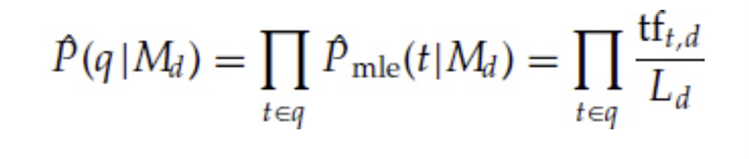
where tf_t,d is the term frequency of term t in document d and L_d is the size of document d. In other words, calculate the fraction of how often each query word appears in document d compared to all words in that document, and then multiply all those fractions with each other.
There are two small problems with the formula above. First, if one of the terms in the query does not appear in a document, the entire probability P(q|d) will be zero. In other words, the only way to get a non-zero probability is if each term in the query appears in the document. The second problem is that the probability of the terms that appear less frequently in the document are likely to be overestimated.
Smoothing techniques
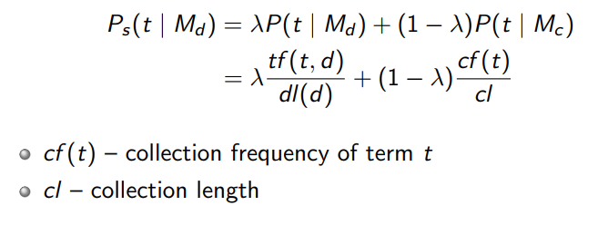
The solution to those mentioned above problems is to introduce smoothing techniques, which will help by creating non-zero probabilities for terms that do not appear in the document, and by creating effective weights to frequent terms. Different smoothing techniques exist such as Jelinek-Mercer smoothing, that uses a linear combination of document-specific and collection-specific maximum likelihood estimations:
Or Dirichlet smoothing:
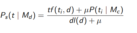
But this is a topic for another blog post.
In summary, traditional term-based retrieval methods are simple to implement and method such as BM25 is one of the most widely used information retrieval functions because of its consistently high retrieval accuracy. However, they deal with the problem based on Bag-of-Words (BoW) representation, thus they only focus on exact syntactic matching and therefore lack the consideration for semantically related words.
By Lan Chu on April 10, 2022.