
Model Explainability - SHAP vs. LIME vs. Permutation Feature Importance
Explaining the way I would explain to my 90 year-old grandmother…
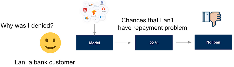
Interpreting complex models helps us understand how and why a model reaches a decision and which features were important in reaching that conclusion, which will aid in overcoming the trust and ethical concerns of using machine learning in making decisions. Choosing the desired model interpretation will generally depend on the answer to three questions: (i) is the model simple enough to offer an intrinsic explanation, (ii) should the interpretable model be model-specific or model-agnostic? and (iii) do we desire local or global explanations?
In this article, we will learn about some post-hoc, local, and model-agnostic techniques for model interpretability. A few examples of methods in this category are PFI Permutation Feature Importance (Fisher, A. et al., 2018), LIME Local Interpretable Model-agnostic Explanations (Ribeiro et al., 2016), and SHAP Shapley Additive Explanations (Lundberg, S. M., & Lee, S. I., 2017). This post will be divided into the following sections:
A. Data introduction
B. Explanation of intuition behind 3 techniques: SHAP, LIME, and Permutation Feature Importance
C. Potential pitfalls
A. Data Introduction
Throughout the article, the models and techniques are applied to real-time series datasets that include: (i) electricity consumption data in the Netherlands in the 2018–2022 period, which is non-public data, and (ii) Weather data in the Netherlands, which is open data from the royal Dutch Meteorology Institute and can be accessed here.
B. The intuition
1. SHAP
SHAP — which stands for Shapley Additive exPlanations, is an algorithm that was first published in 2017 [1], and it is a great way to reverse-engineer the output of any black-box models. SHAP is a framework that provides computationally efficient tools to calculate Shapley values - a concept in cooperative game theory that dates back to 1950.
Game Theory and Machine learning Interpretability
What is the connection between game theory and machine learning interpretability? Instead of having a machine learning problem where we train a model that uses multiple features to create predictions, we now imagine a game where each feature (“player”) collaborates together to obtain a prediction (“score”). Interpreting machine learning now becomes asking the question: how did each player (feature) contribute to obtaining that score (prediction)[2]? The answer is that each feature’s contribution is given by the Shapley value, which tells us how many points we would win or lose if we had played that game without that feature. In other words, the Shapley value helps us explain how to distribute the prediction among features.
Shapley Values
To be a bit more precise, calculating the Shapley value requires knowledge of how the game would have played out for all combinations of players. A unique combination is called a coalition [2]. For example, if we have a game with three players, Alice, Bob & Cheryl, a few valid coalitions would be (Alice) and (Bob, Cheryl). The total number of possible coalitions would be 2 × 2 × 2 = 2^3 = 8 since each player can either be in the game or out. After playing the game with all possible coalitions, we are ready to compute the Shapley value for each player. Let us consider Alice first. The Shapley value for Alice is a weighted sum of the differences in scores that were obtained in games where she was present and in games where she was absent:
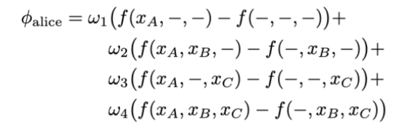
where ωi is a weight that will be explained further below, and − denotes an absent player in that game. For example, f (xA, −, xC ) is a game in Bob’s absence, and f (−, −, −) is a game in which none of the players take part in.
The weights are given by:
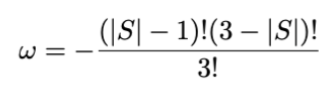
where |S| is the number of players in the coalition, including Alice. For the
four rows in Equation 1 we have |S| = 1, 2, 2, 3 and correspondingly ω1,2,3,4 = 1/3, 1/6, 1/6, 1/3.
Connecting back to explaining machine learning models, we would like to
use Equation (1) to calculate the contribution of a feature in creating a prediction. Typically a model has a fixed input, we all know that a model changes if we drop/add a feature. So calculating Shapley values by searching through all possible feature combinations would mean retraining the model on each of that possible subset of features, which is computationally expensive and perhaps makes zero sense in the real world. We can, however, make an approximation as proposed by the authors of SHAP: removing one or more features from the model is approximately equal to calculating the expectation value of the prediction over all possible values of the features that are removed. Let us look at an example of how this works out.
Imagine we have a model with three features A, B, and C. The prediction we try to explain is, for example, f(5, 3, 10) = 7. One of the steps in obtaining the Shapley values for each feature are, for example, calculating f (5, 3, −). Replacing this with an expectation value is equal to asking ourselves the question: given that xA = 5 and xB = 3, what do we expect the prediction to be? We can take all the possible values of xC from the training set and use those to calculate the expected value. In other words, calculate predictions f(5, 3, xC ) for every value xC from the training set, then take the mean overall predictions. If more than one feature is left out, we have to make a bit more effort, but the principle stays the same. When calculating f(−, −, 10), we ask: what do we expect the model prediction to be when xC = 10? We again take all possible values for xA and xB from the training set but now create all possible pairs of (xA, xB ) before creating all the predictions and calculating the mean. If the training set consists of 100 rows of data, we will have 100 × 100 = 10.000 pairs of values to make predictions. Finally, f (−, −, −) is calculated in a similar fashion. What do we expect the model to predict if we don’t know which values go into it? As before, we take all possible values xA, xB , xC from the training set, create all possible triplets, generate 100 × 100 × 100 = 1.000.000 predictions and calculate the mean. Now that we have approximated the model predictions for every coalition, we can plug those numbers into Equation 1 and obtain the Shapley values for every feature.
Example of SHAP explanation
The last example shows that even for a small training set and a small number of features, it requires calculating a…million predictions. Luckily, there are ways to efficiently approximate the expectation value, which is where SHAP comes into the picture. As mentioned, SHAP is a framework that provides computationally efficient tools to calculate Shapley values. The authors of the SHAP paper proposed KernelSHAP, a kernel-based estimation approach for Shapley values inspired by local surrogate models. They later also proposed TreeSHAP, an efficient estimation approach for tree-based models.
Back to our real data set, we tried to explain the prediction of next-day energy consumption of different neighbourhoods from an Xgboost model using historical/lagged energy consumption, historical/lagged sunshine duration, and geographical location of the neighbourhood. The following figure shows the feature importance of the XGBOOST model from TreeSHAP, which is sorted by the decreasing importance of the features. The color of the horizontal bar shows whether a feature has a positive impact (green) or negative impact (red) on the prediction as compared to the expectation prediction value for a specific instance, in this case, Instance 1.
_Join the_** Medium membership** program to continue learning without limits. I’ll receive a portion of your membership fee if you use the following link, at no extra cost to you. If you decide to do so, thanks a lot!
Join Medium with my referral link — Lan Chu
_Read every story from Lan Chu (and thousands of other writers on Medium). Your membership fee directly supports Lan Chu…_huonglanchu.medium.com
2. LIME
Besides SHAP, LIME is a popular choice for interpreting the black box models. In a previous post, I thoroughly explained what LIME is, how it works, and its potential pitfalls.
Local linearity Assumption
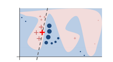
In essence, LIME tries to understand the features that influence the prediction of a black-box model around a single instance of interest. In practice, the decision boundary of a black-box model can look very complex, e.g represented by the blue-pink background in Figure 2. However, studies (Baehrens, David, et al. (2010), Laugel et al., 2018, etc.) have shown that when you zoom in and look at a small enough neighborhood, no matter how complex the model is at a global level, the decision boundary at a local neighborhood can be much simpler, can in fact be even linear.
That said, what LIME does is to go on a very local level and get to a point where it becomes so local that a linear model is powerful enough to explain the behavior of the black-box model at that locality [4]. You choose an instance X0 to explain, LIME will generate new fake instances around this instance X0 by sampling a neighborhood around this selected instance. Next, it applies the original black-box model on the permuted instances to generate the corresponding predictions and weights those generated instances by their distances to the explained instance. The weights are determined by a kernel function which takes Euclidean distances and kernel width as input and outputs the importance score (weight) for each generated instance.
In this obtained dataset (which includes the generated instances, the corresponding predictions, and the weights), LIME trains an interpretable model (e.g, linear model) which captures the behaviors of the complex model in that neighborhood. The coefficients of that local linear model will tell us which features drive the prediction to one way or the other and, most importantly, at that locality.
Example of LIME Explanation
Similar to SHAP, the output of LIME is a list of explanations, reflecting the contribution of each feature value to the model prediction.
3. Permutation Feature Importance (PFI)
Decrease in Model Performance
The idea behind PFI is simple. It measures the decrease in model performance (e.g RMSE) after we shuffled the feature’s values and therefore explains which features wrongly drive the model’s performance [5]. Simply put, a feature is important if shuffling its values increases the model error because in this case, the model relied on the feature for the prediction. A feature is not-so-important if shuffling its values leaves the model error unchanged because in this case, the model ignores the feature for the prediction [2]. As an example, let’s assume a model with RMSE equal to 42 on the validation set. If you shuffle one feature, the validation RMSE goes up to 47, this means the importance of this feature is then 5.
Example of PFI Explanation
Back to our real example, the explanation of PFI says the geographical location features (Location A, Location B, Location C) play the most important roles, having the largest impact on the increase in model error. This is very different from the explanation of SHAP and LIME, but it perhaps can be explained. Because we are looking at time series data, the lagged features are highly correlated, e.g, the sunshine duration of one week ago (sunshine_lag7) is correlated with sunshine duration 6 days ago (sunshine_lag6). Let’s say we now shuffle the feature sunshine_lag7. When two features are correlated, and one of the features is permuted, the model still has access to the information inside this feature through its correlated feature, and the model can now rely on sunshine_lag6 measurement. This results in a lower importance value for both features, where they might actually be important. This is exactly what happened in this case.
C. Potential Pitfalls
The PFI method explains which features drive the model’s performance (e.g. RMSE) while methods such as LIME and SHAP explain which features played a more important role in generating a prediction.
SHAP is probably state-of-the-art in Machine Learning Explain-ability. It has a clear interpretation and a solid foundation in game theory. The Shapley value might be the only method that delivers a full explanation because it is based on a solid theory and distributes the effects fairly by calculating the difference between the prediction of the model when adding the feature values and the expectation prediction when the feature value is absent. The downside of SHAP is that the Shapley value requires a lot of computing time because the training time grows exponentially with the number of features. One solution to keep the computation time manageable is to compute contributions for only a few samples of the possible coalitions [2]. Another limitation is that, for a single instance, the Shapley value returns a single Shapley value per feature value, it does not give the prediction model like what LIME does. This means it cannot be used to make statements about changes in prediction for changes in the input.
LIME’s explanation is rather straightforward. However, it requires defining a neighborhood and is shown sometimes to be unstable and easily manipulable. The instability of the LIME explanation comes from the fact that it depends on the number of instances that are generated and the chosen kernel width, which determines how large or small the neighborhood is. This neighborhood defines the locality level of the explanation. A purposeful neighborhood needs to be small enough to achieve the local linearity but large enough to avoid the threat of under-sampling or bias toward a global explanation. In some scenarios, you can change the explanation’s direction by changing the kernel width. Methods like LIME are based on the assumption that things will have a linear relationship at the local level, but there is no theory as to why this should work. At times when your black-box model is extremely complex, and the model is simply not locally linear, a local explanation using a linear model will not be good enough. LIME would probably be able to give a good local explanation — provided that the right neighborhood and the local linearity are achieved.
Permutation feature importance is linked to the error of the model, which is not always what you want. PFI is also badly suited for models that are trained with correlated features, as adding a correlated feature can decrease the importance of the associated feature by splitting the importance between both features. This often will lead to misleading interpretations, as explained above, and are therefore not suitable to explain time series models or when there are strongly correlated features.
References
[1] [SHAP main paper (2017)] A Unified Approach to Interpreting Model Predictions: http://papers.nips.cc/paper/7062-a-unified-approach-to-interpreting-model-predictions.pdf
[2] [Book] Interpretable Machine Learning: https://christophm.github.io/interpretable-ml-book/shap.html
[3] SHAP Package: https://github.com/slundberg/shap
[4] Ribeiro, M. T., Singh, S., & Guestrin, C. (2016, August). “ Why should i trust you?” Explaining the predictions of any classifier. In Proceedings of the 22nd ACM SIGKDD international conference on knowledge discovery and data mining (pp. 1135–1144).
[5] Altmann, A., Toloşi, L., Sander, O., & Lengauer, T. (2010). Permutation importance: a corrected feature importance measure. Bioinformatics, 26(10), 1340–1347.
[6] https://towardsdatascience.com/shap-explained-the-way-i-wish-someone-explained-it-to-me-ab81cc69ef30
By Lan Chu on July 22, 2022.
Exported from Medium on January 7, 2023.