What do countries talk about at the UN General Debate — Topic modelings using LDA.

The intuition behind LDA and its limitations, along with python implementation using Gensim.

By Lan Chu and Robert Jan Sokolewicz.

[Find the code for this article here.]

1. What is Latent Dirichlet Allocation?

Latent Dirichlet Allocation (LDA) is a popular model when it comes to analyzing large amounts of text. It is a generative probabilistic model that enables users to uncover hidden (“latent”) topics and themes from a collection of documents. LDA models each document as being generated by a process of repeatedly sampling words and topics from statistical distributions. By applying clever algorithms, LDA is able to recover the most likely distributions that were used in this generative process (Blei, 2003). These distributions tell us something about which topics exist and how they are distributed among each document.

Let us first consider a simple example to illustrate some of the key features of LDA. Imagine we have the following collection of 5 documents

• 🍕🍕🍕🍕🍕🦞🦞🦞🐍🐍🐋🐋🐢🐌🍅
• 🐌🐌🐌🐌🐍🐍🐍🐋🐋🐋🦜🦜🐬🐢🐊
• 🐋🐋🐋🐋🐋🐋🐢🐢🐢🐌🐌🐌🐍🐊🍕
• 🍭🍭🍭🍭🍭🍭🍕🍕🍕🍕🍅🍅🦞🐍🐋
• 🐋🐋🐋🐋🐋🐋🐋🐌🐌🐌🐌🐌🐍🐍🐢

and wish to understand what kind of topics are present and how they are distributed between documents. A quick observation shows us we have a lot of food and animal-related emojis

• food: {🍕,🍅,🍭,🦞}
• animal: {🦞🐍🐋🐬🐌🦜}

and that these topics appear in different proportions in each document. Document 4 is mostly about food, document 5 is mostly about animals, and the first three documents are a mixture of these topics. This is what we refer to when we talk about topic distribution, the proportion of topics is distributed differently in each document. Furthermore, we see that the emojis 🐋 and 🍭 appear more frequently than other emojis. This is what we refer to when we talk about the word distribution of each topic.

These distributions for topics and words in each topic are exactly what is returned to us by LDA. In the above example, we labeled each topic as food and animal, something that LDA, unfortunately, does not do for us. It merely returns us the word distribution for each topic, from which we - as users have to make an inference on what the topic actually means.

So how does LDA achieve the word distribution for each topic? As mentioned, it assumes that each document is produced by a random process of drawing topics and words from various distributions, and uses a clever algorithm to look for parameters that are the most likely parameters to have produced the data.

2. Intuition behind LDA

LDA is a probabilistic model that makes use of both Dirichlet and multinomial distributions. Before we continue with the details of how LDA uses these distributions, let us make a small break to refresh our memory on what these distributions mean. The Dirichlet and multinomial distributions are generalizations of Beta and binomial distributions. While Beta and binomial distributions can be understood as random processes involving flipping coins (returning discrete value), Dirichlet and Multinomial distributions deal with random processes dealing with e.g. throwing dice. So, let us take a step back and consider the slightly simpler set of distributions: beta distribution and binomial distribution.

2.1 Beta and binomial distribution

To make it simple, we will use an example of a coin flip to illustrate how LDA works. Imagine that we have a document that is entirely written with only two words: 🍕 and 🍅, and that the document is generated by repeatedly flipping a coin. Each time the coin lands heads we write 🍕, and each time the coin lands tails we write 🍅. If we know beforehand what the bias of the coin is, in other words, how likely it is to produce 🍕, we can model the process of generating a document using a binomial distribution. The probability of producing 🍕🍕🍕🍕🍕🍕🍕🍅🍅🍅 (in any order) for example is given by P = 120P(🍕)⁷P(🍅)³, where 120 is the number of combinations to arrange 7 pizzas and 3 tomatoes.

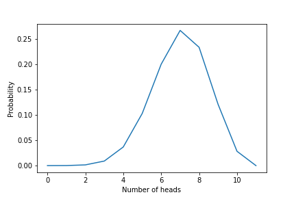
But how do we know the probabilities P(🍕) and P(🍅)? Given the above document, we might estimate P(🍕) = 7/10 and P(🍅)= 3/10, but how certain are we in assigning those probabilities? Flipping the coin 100 or even 1000 times would narrow down these probabilities more.

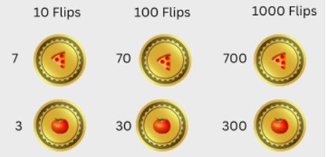
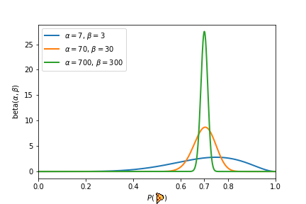
In the above experiment, each experiment would give us the same probability of P(🍕)=7/10 = 0.7. Each subsequent experiment, however, would strengthen our beliefs that P(🍕)=7/10. It is the beta distribution that gives us a way to quantify this strengthening of our beliefs after seeing more evidence. The beta distribution takes two parameters 𝛼 and 𝛽 and produces a probability distribution of probabilities. The parameters 𝛼 and 𝛽 can be seen as “pseudo-counts” and represents how much prior knowledge we have about the coin. Lower values of 𝛼 and 𝛽 lead to a distribution that is wider and represents uncertainty and lack of prior knowledge. On the other hand, larger values of 𝛼 and 𝛽 produce a distribution that is sharply peaked around a certain value (e.g. 0.7 in the third experiment). This means we can back up our statement that P(🍕)=0.7. We illustrate the beta distribution that corresponds to the above three experiments in the figure below.

Now think of it this way, we have a prior belief that the probability of landing head is 0.7. This is our hypothesis. You continue with another experiment — flipping the coin 100 times and getting 74 heads and 26 tails, what is the probability that the prior probability equal to 0.7 is correct? Thomas Bayes found that you can describe the probability of an event, based on prior knowledge that might be related to the event through Bayes theorem, which shows how given some likelihood, and a hypothesis and evidence, we can obtain the posterior probability:

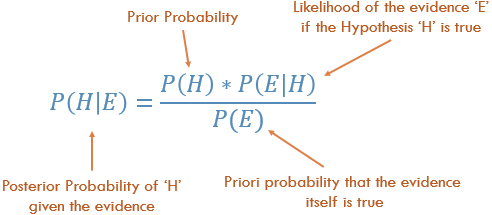
There are 4 components here:

• Prior Probability: The hypothesis or prior probability. It defines our prior beliefs about an event. The idea is that we assume some prior distribution, the one that is most reasonable given our best knowledge. Prior probability is the P(Head) of each coin, generated by using beta distribution, which in our example is 0.7
• Posterior Probability: The probability of the prior probability given the evidence. It is a probability of probability. Given 100 flips with 74 heads and 26 tails, what is the probability that the prior probability equal to 0.7 is correct? In other words, with evidence/observed data, what is the probability that the prior belief is correct?
• Likelihood: The likelihood can be described as the probability of observing the data/evidence given that our hypothesis is true. For example, let’s say I flipped a coin 100 times and got 70 heads and 30 tails. Given our prior belief that the P(Head) is 0.7, what is the likelihood of observing 70 heads and 30 tails out of 100 flips? We will use the binomial distribution to quantify the Likelihood. The binomial distribution uses the prior probability from the beta distribution (0.7) and the number of experiments as input and samples the number of heads/tails from a binomial distribution.
• Probability of the Evidence: Evidence is the observed data/result of the experiment. Without knowing what the hypothesis is, how likely is it to observe the data? One way of quantifying this term is by calculating P(H)*P(E|H) for every possible hypothesis and taking the sum. Because the evidence term is in the denominator, we see an inverse relationship between the evidence and posterior probability. In other words, having a high probability of evidence leads to a small posterior probability and vice versa. A high probability of evidence reflects that alternative hypotheses are as compatible with the data as the current one so we cannot update our prior beliefs.

2.2 Document and topic modeling

Think of it this way: I want to generate a new document using some mathematical frameworks. Does that make any sense? If it does, how can I do that? The idea behind LDA is that each document is generated from a mixture of topics and each of those topics is a distribution over words (Blei, 2003). What you can do is randomly pick up a topic, sample a word from that topic, and put the word in the document. You repeat the process, pick up the topic of the next word, sample the next word, put it in the document…and so on. The process repeats until done.

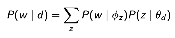
Following the Bayesian theorem, LDA learns how topics and documents are represented in the following form:

There are two things that are worth mentioning here:

• First, a document consists of a mixture of topics, where each topic z is drawn from a multinomial distribution z~Mult(θ) (Blei et al., 2003)

Let’s call Theta (θ) the topic distribution of a given document, i.e the probability of each topic appearing in the document. In order to determine the value of θ, we sample a topic distribution from a Dirichlet distribution. If you recall what we learned from beta distribution, each coin has a different probability of landing heads. Similarly, each document has different topic distributions, which is why we want to draw the topic distributions θ of each document from a Dirichlet distribution. Dirichlet distribution using alpha/α — proper knowledge/hypothesis as the input parameter to generate topic distribution θ, that is θ ∼ Dir(α). The α value in Dirichlet is our prior information about the topic mixtures for that document. Next, we use θ generated by the Dirichlet distribution as the parameters for the multinomial distribution z∼Mult(θ) to generate the topic of the next word in the document.

• Second, each topic z consists of a mixture of words, where each word is drawn from a multinomial distribution w~Mult(ϕ) (Blei et al., 2003)

Let’s call phi (ϕ) the word distribution of each topic, i.e. the probability of each word in the vocabulary appearing in a given topic z. In order to determine the value of ϕ, we sample a word distribution of a given topic from a Dirichlet distribution φz ∼ Dir(β) using beta as the input parameter β — the prior information about the word frequency in a topic. For example, I can use the number of times each word was assigned for a given topic as the β values. Next, we use phi (ϕ) generated from Dir(β) as the parameter for the multinomial distribution to sample the next word in the document — given that we already knew the topic of the next word.

The whole LDA generative process for each document is as followed:

p(w,z,θ,ϕ | α, β ) = p(θ| α)* p(z| θ) * p(ϕ| β) *p(w| ϕ)

To summarize, the first step is getting the topic mixtures of the document — θ generated from Dirichlet distribution with the parameter α. That gives us the first term. The topic z of the next word is drawn from a multinomial distribution with the parameter θ, which gives us the second term. Next, the probability of each word appearing in the document ϕ is drawn from a Dirichlet distribution with the parameter β, which gives third term p(ϕ|β). Once we know the topic of the next word z, we use the multinomial distribution using ϕ as a parameter to determine the word, which gives us the last term.

3. Python Implementation with Gensim

3.1 The data set

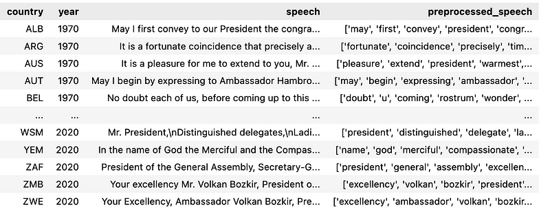
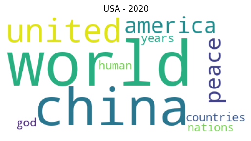
The LDA python implementation in this post uses a dataset composed of the corpus of texts of UN General Debate . It contains all the statements made by each country’s presentative at UN General Debate from 1970 to 2020. The data set is open data and is available online here. You can gain extra insight into its contents by reading this paper.

3.2 Preprocessing the data

As part of preprocessing, we will use the following configuration:

• Lower case
• Tokenize (split the documents into tokens using NLTK tokenization).
• Lemmatize the tokens (WordNetLemmatizer() from NLTK)
• Remove stop words

3.3 Training a LDA Model using Gensim

Gensim is a free open-source Python library for processing raw, unstructured texts and representing documents as semantic vectors. Gensim uses various algorithms such as Word2Vec, FastText, Latent Semantic Indexing LSI, Latent Dirichlet Allocation LDA etc… It will discover the semantic structure of documents by examining statistical co-occurrence patterns within a corpus of training documents.

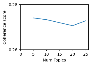
Regarding the training parameters, first of all, let’s discuss the elephant in the room: how many topics are there in the documents? There is no easy answer to this question, it depends on your data and your knowledge of the data, and how many topics you actually need. I randomly used 10 topics since I wanted to be able to interpret and label the topics.

Chunksize parameter controls how many documents are processed at a time in the training algorithm. As long as the chunk of documents fits into memory, increasing the chunksize will speed up the training. Passes control how often we train the model on the entire corpus, which is known as epochs. Alpha and eta are the parameters as explained in sections 2.1 and 2.2. The shape parameter eta here corresponds to beta.

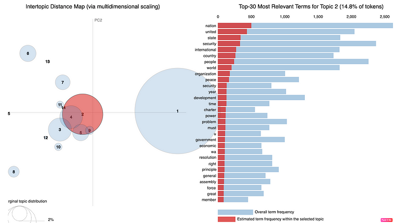
In the result of the LDA model as below, let us look at topic 0, as an example. It says 0.015 is the probability the word “nation” will be generated/appear in the document. This means if you draw the sample an infinite amount of times, then the word “nation” will be sampled 0.015% of the time.

topic #0 (0.022): 0.015*“nation” + 0.013*“united” + 0.010*“country” + 0.010*“ha” + 0.008*“people” + 0.008*“international” + 0.007*“world” + 0.007*“peace” + 0.007*“development” + 0.006*“problem”

topic #1 (0.151): 0.014*“country” + 0.014*“nation” + 0.012*“ha” + 0.011*“united” + 0.010*“people” + 0.010*“world” + 0.009*“africa” + 0.008*“international” + 0.008*“organization” + 0.007*“peace”

topic #2 (0.028): 0.012*“security” + 0.011*“nation” + 0.009*“united” + 0.008*“country” + 0.008*“world” + 0.008*“international” + 0.007*“government” + 0.006*“state” + 0.005*“year” + 0.005*“assembly”

topic #3 (0.010): 0.012*“austria” + 0.009*“united” + 0.008*“nation” + 0.008*“italy” + 0.007*“year” + 0.006*“international” + 0.006*“ha” + 0.005*“austrian” + 0.005*“two” + 0.005*“solution”

topic #4 (0.006): 0.000*“united” + 0.000*“nation” + 0.000*“ha” + 0.000*“international” + 0.000*“people” + 0.000*“country” + 0.000*“world” + 0.000*“state” + 0.000*“peace” + 0.000*“organization”

topic #5 (0.037): 0.037*“people” + 0.015*“state” + 0.012*“united” + 0.010*“imperialist” + 0.010*“struggle” + 0.009*“aggression” + 0.009*“ha” + 0.008*“american” + 0.008*“imperialism” + 0.008*“country”

topic #6 (0.336): 0.017*“nation” + 0.016*“united” + 0.012*“ha” + 0.010*“international” + 0.009*“state” + 0.009*“world” + 0.008*“country” + 0.006*“organization” + 0.006*“peace” + 0.006*“development”

topic #7 (0.010): 0.020*“israel” + 0.012*“security” + 0.012*“resolution” + 0.012*“state” + 0.011*“united” + 0.010*“territory” + 0.010*“peace” + 0.010*“council” + 0.007*“arab” + 0.007*“egypt”

topic #8 (0.048): 0.016*“united” + 0.014*“state” + 0.011*“people” + 0.011*“nation” + 0.011*“country” + 0.009*“peace” + 0.008*“ha” + 0.008*“international” + 0.007*“republic” + 0.007*“arab”

topic #9 (0.006): 0.000*“united” + 0.000*“nation” + 0.000*“country” + 0.000*“people” + 0.000*“ha” + 0.000*“international” + 0.000*“state” + 0.000*“peace” + 0.000*“problem” + 0.000*“organization”

3.4 Quality of the topics

The topics that are generated are typically used to tell a story. Good quality topics, then, are those that are easily interpretable by humans. A popular metric to assess topic quality is coherence, where larger coherence values generally correspond to more interpretable topics. This means we could use the topic coherence scores to determine the optimal number of topics. Two popular coherence metrics are the UMass and word2vec coherence scores. UMass calculates how often two words in a topic appear in the same document, relative to how often they appear alone. Having a topic with words such as United, Nations, and States would have a lower coherence score because even though United often co-appears with Nations and States in the same document, Nations and States do not. Coherence scores based on word2vec on the other hand, take a different approach. For each pair of words in the topic, word2vec will vectorize each word and compute the cosine similarity. The cosine similarity score tells us if two words are semantically similar to each other.

4. Limitations

• Order is irrelevant: LDA processes documents as a ‘bag of words’. A bag of words means you view the frequency of the words in a document with no regard for the order the words appeared in. Obviously, there is going to be some information lost in this process, but our goal with topic modeling is to be able to view the ‘big picture’ from a large number of documents. An alternate way of thinking about it: I have a vocabulary of 100k words used across 1 million documents, then I use LDA to look at 500 topics.
• The number of topics is a hyperparameter that needs to be set by the user. In practice, the user runs LDA a few times with different numbers of topics and compares the coherence scores for each model. Higher coherence scores typically mean that the topics are better interpretable by humans.
• LDA does not always work well with small documents such as tweets and comments.
• Topics generated by LDA aren’t always interpretable. In fact, research has shown that models with the lowest perplexity or log-likelihood often have less interpretable latent spaces (Chang et al 2009).
• Common words often dominate each topic. In practice, this means removing stop words from each document. These stop words can be specific to each collection of documents and will therefore be needed to construct by hand.
• Choosing the right structure for the prior distribution. In practice, packages like Gensim opt for a symmetric Dirichlet by default. This is a common choice and does not appear to lead to worse topic extraction in most cases (Wallach et al 2009, Syed et al 2018).
• LDA does not take into account correlations between topics. For example “cooking” and “diet” are more likely to coexist in the same document, while “cooking” and “legal” would not (Blei et al 2005). In LDA topics are assumed to be independent of each other due to the choice of using the Dirichlet distribution as a prior. One way to overcome this issue is by using correlated topic models instead of LDA, which uses a logistic normal distribution instead of a Dirichlet distribution to draw topic distributions.

Thank you for reading. If you find my post useful and are thinking of becoming a Medium member, you can consider supporting me through this Referred Membership link :) I’ll receive a portion of your membership fee at no extra cost to you. If you decide to do so, thanks a lot!

References:

1. Blei, David M., Andrew Y. Ng, and Michael I. Jordan. “Latent dirichlet allocation.” Journal of machine Learning research 3.Jan (2003): 993–1022.
2. The little book of LDA. An overview of LDA and Gibs sampling. Chris Tufts.
3. Chang, Jonathan, Sean Gerrish, Chong Wang, Jordan Boyd-Graber, and David Blei. “Reading tea leaves: How humans interpret topic models.” Advances in neural information processing systems 22 (2009).
4. Lafferty, John, and David Blei. “Correlated topic models.” Advances in neural information processing systems 18 (2005).
5. Wallach, Hanna, David Mimno, and Andrew McCallum. “Rethinking LDA: Why priors matter.” Advances in neural information processing systems 22 (2009).
6. Hofmann, Thomas. “Probabilistic latent semantic analysis.” arXiv preprint arXiv:1301.6705 (2013).
7. Syed, Shaheen, and Marco Spruit. “Selecting priors for latent Dirichlet allocation.” In 2018 IEEE 12th International Conference on Semantic Computing (ICSC), pp. 194–202. IEEE, 2018.
8. https://dataverse.harvard.edu/file.xhtml?fileId=4590189&version=6.0
9. Beta Distribution

Beta distribution - Wikipedia
_In probability theory and statistics, the beta distribution is a family of continuous probability distributions defined…_en.wikipedia.org

By Lan Chu on November 8, 2022.

Canonical link