What is Biological Neuron?

The whole purpose of Artificial Neural Networks is to look at the human brain’s architecture in the hope that we can mimic how a human brain works and build such an intelligent artificial learning mechanism. First let’s talk about the biological neurons which are the basic building blocks of the human brain and nervous system. An easy way to understand the structure of neuron is thinking of it as a tree. Basically, a neuron contains three main parts: a cell body where the nucleus lies, many small branches called dendrites, plus a long extension called the axon. These three components can be respectively represented as the trunk (cell body), the branches (dendrites) and root (axon) of a tree.

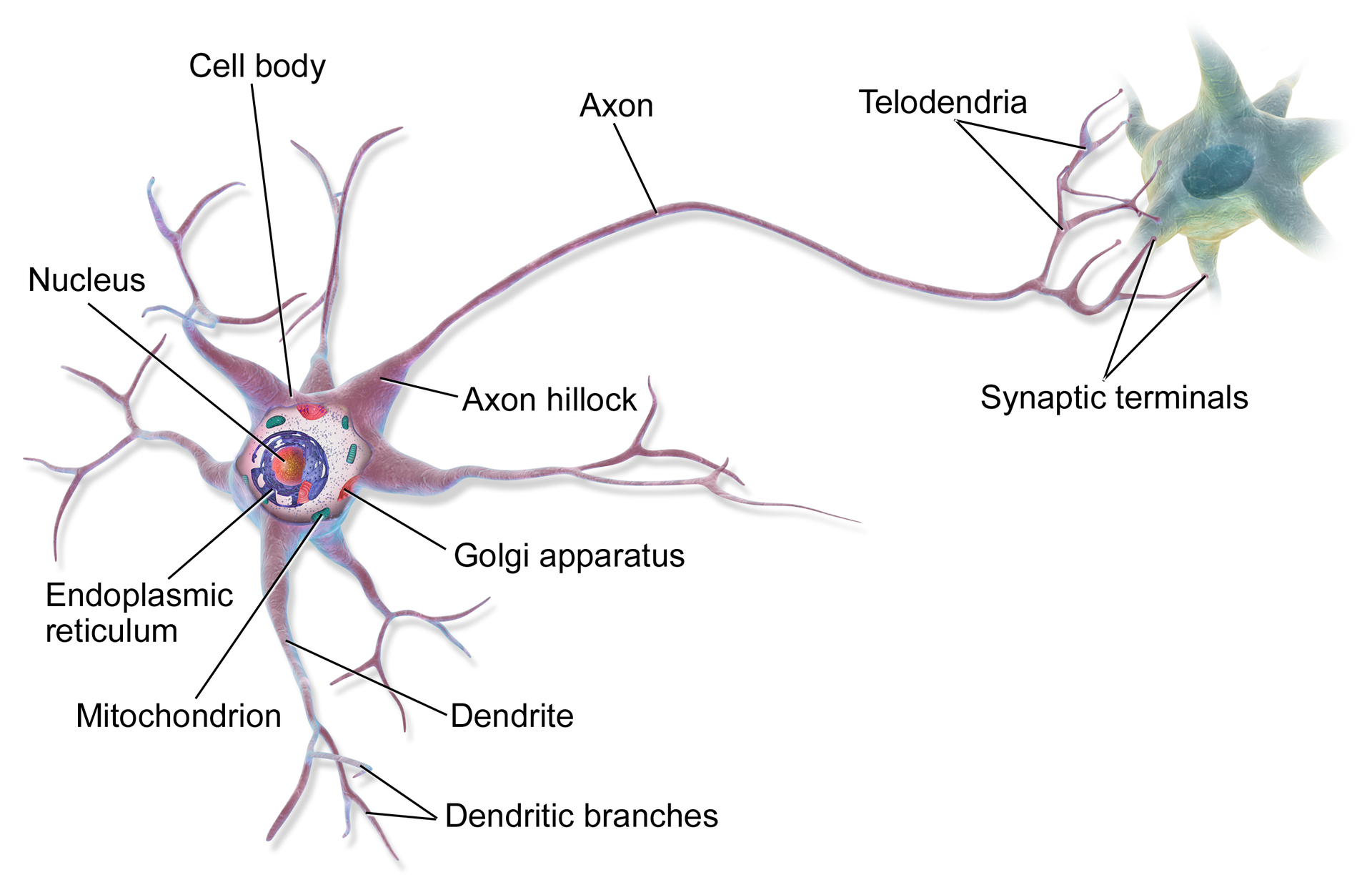
How it works conceptually is that the dendrites are connected to axons of other neurons. Dendrites receive the signal for the neuron while the axon is the transmitter of the signal. Biological neurons are organized in a huge network of billions of neurons, each neuron typically connected to thousands of other neurons. When a neuron wants to talk to another neuron, it sends an electrical message throughout the entire axon. If a neuron receives a sufficient number of signals from other neurons, it produces its own signals.

From Biological to Artificial Neuron

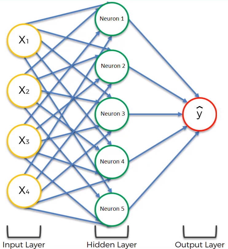
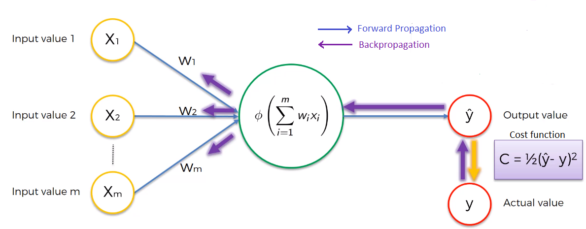
Now, let’s move from biological neurons to artificial neurons. The architecture of artificial neuron also has input signal and an output signal and it will simply activate the output when the input is activated. Just like how the human’s brain receives sensory information to understand and perceive the world through five basic senses: Touch, Sight, Sound, Smell and Taste, artificial neurons receive images, sounds, tabular data, etc. as input values. The Perceptron is one of the simplest ANN architectures, which has only one input and one output layer. Each input is associated with a weight. The artificial neural network will compute a weighted sum of its input and output the result. Multi-layer perceptron meanwhile is composed of one input layer, one or more hidden layers (which is connected to the input layer), and one final layer called the output layer which outputs the predicted value ŷ. In the example below, we present an ANN with one hidden layer, and five neurons in the hidden layers. Before the neural network is trained, it will have all the possible synapses and contain a total of 25 weights (20 between the input and hidden layer and 5 between the hidden layer and output layer)

Let’s take an example to further understand how ANN works. Let’s say you work for a Bank and you are supplied with data about the bank’s customers called X1, X2, X3, X4 which are customer income, age, loan amount, interest rate respectively. Now as a bank, your business problem would be: given a customer profile, can I predict which customers are going to default? The idea is that you call the neural network architecture, you give the network thousands of observations which have already been categorized (default or not) and let the neural network go and learn the features of default and non-default customers and when you give the network new customer data, it will be able to tell which one will or will not default. What happens in details is:

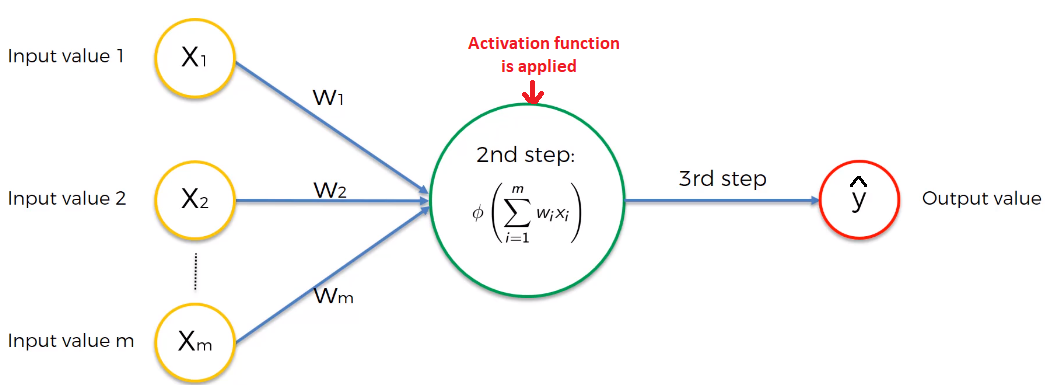
1. First, the neural network takes the weighted sum of all of the input values.

2. Forward propagation

In the hidden layer, the activation function which takes into account the input and weight of each input is applied in each neuron and produces an output which serves as new input for the next layer. As such, the result of the previous layer is passed on to the next layer, its output is computed and again passed to the next layer. The process continues until when we get the output of the output layer, which is also the last layer in a neural network architecture. The output value of this layer is also the predicted value — ŷ of the model.

3. Backpropagation process

Now, we have an output ŷ and the network is going to start the backpropagation process. It all has to do with the so-called loss function. In essence, a loss function is a function that compares the predicted output and the actual output of the network and returns the error information.

For each training instance the backpropagation measures how each weight in the network contributes to the overall error by feeding the error information (differences between y and ŷ) back through the network. This allows the model to update the weights using optimization algorithm. Essentially, what this algorithm does is tweaking all the weights in the network until when the loss function is minimized. This means your final neural network is ready because you have found the optimal weight where the error is minimized. Among optimization algorithms, Gradient-Descent-based is the simplest and most widely used neural network optimization algorithm. To understand how exactly the weights are adjusted using Gradient Descent, a detailed explanation can be found here. You can also gain some insights for alternatives of Gradient Descent in this post.

Actual Implementation

Assuming you installed Jupiter and ScikitLearn, you can simply use pip or conda to install TensorFlow.

Part 1. Loading data and data processing

I use this data set of loan default on Hackereath. Since it was a quite large dataset, I only make use of the training set as my full dataset for this example. Basically, we have a dataset of a bank, which contains information about its customers. The size is around 500.000 observations and among all the features in that data set, I picked up those which have the highest correlation with the target variable (default or non-default) to train the model. Certain data processing has been done before training the model. For example, since we are going to train the neural network, we must scale the input features. Find a detail description of all the steps taken on my Github repo.

#Importing the libraries

import pandas as pd
import tensorflow as tf
from tensorflow import keras
import pandas as pd
import numpy as np
from sklearn import preprocessing, metrics
import matplotlib.pyplot as plt
from sklearn import preprocessing
from sklearn.model_selection import KFold
import re
import timeit
import random
random.seed(3)
import seaborn as sns
from tqdm.notebook import tqdm

#Loading data and some data processing

sns.heatmap(data = df.corr(),annot=True, linewidths=1.5, fmt='.1g',cmap=plt.cm.Reds)
plt.show()
df = df[['funded_amnt_inv', 'term', 'int_rate', 'home_ownership', 'annual_inc','total_rec_int','tot_cur_bal','loan_status']]
df = df.dropna()
df['term'] = df['term'].apply(lambda x: np.int(x[:2]))
target= df['loan_status'].values
df.drop('loan_status', axis = 1, inplace = True)
from sklearn.compose import ColumnTransformer
from sklearn.preprocessing import OneHotEncoder
ct = ColumnTransformer(transformers=[('encoder', OneHotEncoder(), [3])], remainder='passthrough')
X = np.array(ct.fit_transform(df.values))
y = target

Part 2. Building the ANN

Now let’s build the neural network! I am going to create a classification Multi-layer Perceptron with one hidden layers.

1. Creating ANN

First, we need to create an ANN which is a Sequential model. In essence, sequential models are composed of multiple layers, connected sequentially. For an ANN, it will contain an input layer, hidden layer(s) and an output layer.

#Initialize ANN
ann = tf.keras.models.Sequential()

Next, we need to add input layer and hidden layer(s) using the Dense class. Each Dense layer manages its own weight matrix, containing all the connection weights between the neurons and their inputs. In this case, I specify the Dense hidden layer with 12 neurons. So, the question is, how do we know how many neurons should there be? Unfortunately, there is not really a rule of thumb, it is just a matter of trials and errors. And don’t forget the Activation function. For a fully connected ANN, we need to use the rectified function — ‘Relu’.

#Adding the input layer and the first hidden layer
ann.add(tf.keras.layers.Dense(units=12, activation='relu'))

#Adding the second hidden layer
ann.add(tf.keras.layers.Dense(units=12, activation='relu'))

Finally, we add a Dense output layer. For a binary classification problem, we just need a single output neuron using the “sigmoid” activation function in the output layer. That’s why the unit is set equal to 1. The output will be a number between 0 and 1, which you can interpret as the estimated probability of the positive class.

#Adding output layer
ann.add(tf.keras.layers.Dense(units=1, activation='sigmoid'))

2. Compiling ANN

After the model is created, you must specify the loss function and the optimizer you want to use as well as the list of metrics for training and evaluating the model using the compile() method

# Compiling the ANN
ann.compile(optimizer = 'adam', loss = 'binary_crossentropy', metrics = ['accuracy', keras.metrics.Recall(),keras.metrics.Precision()])

There are multiple optimizer functions, Here I choose ‘Adam’ function. You can also choose others, Stochastic Gradient Descent for instance. Since this is a classifier, we would use the “binary_crossentropy” as loss function. Now congratulations! You have just built your very first artificial brain. Let’s move to training our model.

Part 3. Training the ANN

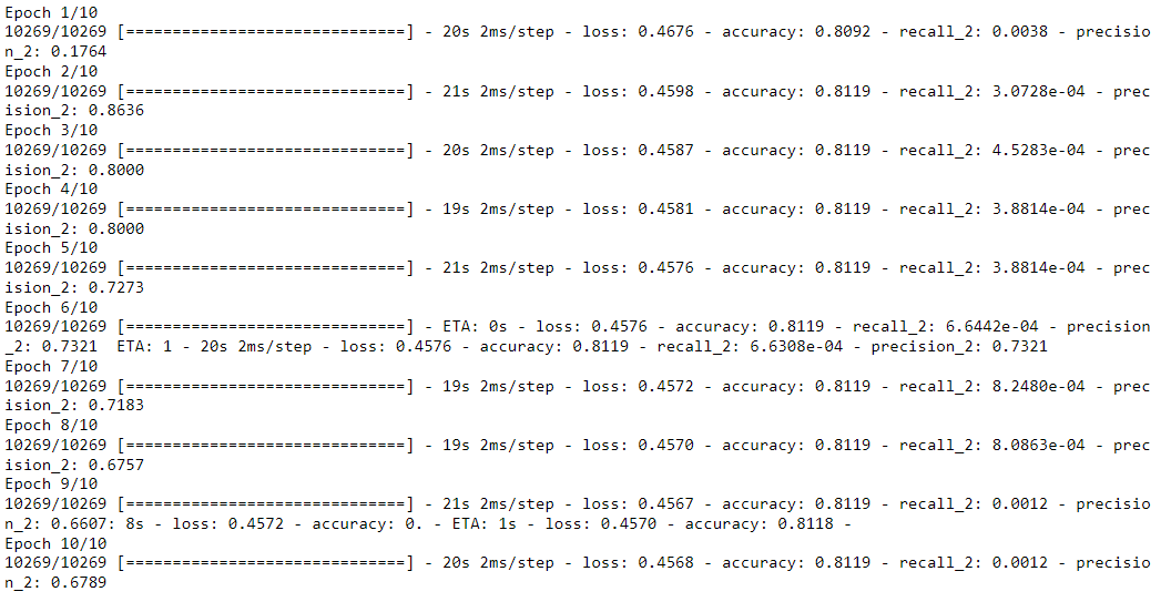
Now the model is ready to be trained. For this we simply need to call its fit() method. We pass the input features (X_train) and the target classes (y_train), as well as the number of epochs — which is the number of times you train your ANN on the entire training set to the model. And that’s it! The neural network is now being trained. At each epoch during training, Keras displays the number of instances processed so far, the mean training time per sample, accuracy and other extra metrics you asked for on the training set. You can see that the training loss went down with each epoch which means the network learns the training data better and better with each epoch. 81% the accuracy does not sound too bad but this is simply because in the training dataset, only about 15% of the customers are default, so if your model always guess that a customer are not going to default, it will be right about 85% of the time!! This explains why accuracy is not always the preferred performance measure for classifiers, especially when your dataset is skewed i.e., when one classes are much more frequent than other. As it shows below, unfortunately, the recall of my model is extremely low.

#Training the ANN 
ann.fit(X_train, y_train, batch_size = 32, epochs = 10)

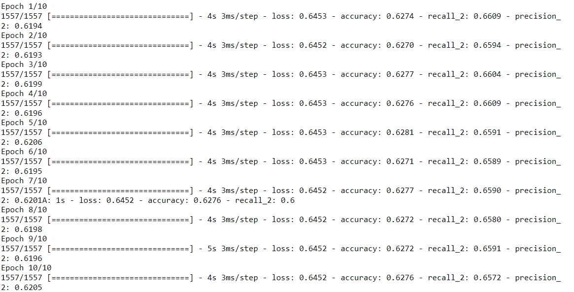
As previously mentioned, my training set was very skewed, with class non-default being overrepresented so I decide to down-sample the non-default class to have a more balanced dataset, let’s say 50–50.

# Downsample the trainingset to have more balanced training data
x0 = X_train[y_train==0]
x1 = X_train[y_train==1]
np.random.shuffle(x0)
x0 = x0[:62256]
x_train_downsample = np.concatenate([x0, x1])
y_train_downsample = np.concatenate([62256*[0], 62256*[1]])

Next, I retrained the model using the down-sampled dataset. Now you see that even though there are not many differences in accuracy, recall increases significantly compared to the previous training, which is a great sign. So congratulations! Your model can be improved tremendously just by balancing your training data.

#Retrain the model using the down-sampled dataset
ann.fit(x_train_downsample, y_train_downsample, batch_size = 32, epochs = 10)

Part 4. Making prediction and evaluating the ANN Once you are satisfied with your model, you should evaluate it on the test set which can be easily done by calling the model’s predict() method to make predictions:

#Make the predictions and output accuracy, precision and recall
y_pred = ann.predict(X_test)
y_pred = (y_pred > 0.55)
print(np.concatenate((y_pred.reshape(len(y_pred),1), y_test.reshape(len(y_test),1)),1))
As mentioned above, accuracy is generally not the preferred performance measure for classifiers, a much better way to evaluate the performance of a classifier is to look at the confusion matrix. The idea is to count the number of times instances of class 1 are classified as class 0. You can find here a detailed explanation of the confusion matrix.
from sklearn.metrics import confusion_matrix, accuracy_score
def conf_matrix(y,pred):
    ((tn, fp), (fn, tp)) = metrics.confusion_matrix(y, pred)
    ((tnr,fpr),(fnr,tpr))= metrics.confusion_matrix(y, pred, 
            normalize='true')
    display(pd.DataFrame([[f'TN = {tn} (TNR = {tnr:1.2%})', 
                                f'FP = {fp} (FPR = {fpr:1.2%})'], 
                         [f'FN = {fn} (FNR = {fnr:1.2%})', 
                                f'TP = {tp} (TPR = {tpr:1.2%})']],
            index=['True 0', 'True 1'], 
            columns=['Pred 0', 
                            'Pred 1']))
    print("precision: {}".format(precision_score(y_test, y_pred)))
    print("recall: {}".format(recall_score(y_test, y_pred)))
    
conf_matrix(y_test,y_pred)

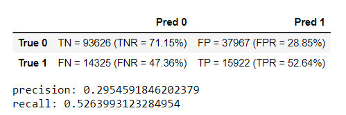
Using the components of the confusion matrix we can construct two metrics called the precision and recall:

Precision = TP / (TP + FP)

Recall = TP / (TP + FN)

Precision answers the question “of all the defaults the model predicts, which fraction of them was correct?”, whereas recall answers the question “of all the defaults, which fraction was correctly identified as default?” One way to have perfect precision is to make one single positive prediction and ensure it is completely correct (precision = 100%). This, however, would not be useful since the classifier will ignore all but one positive instance. That’s why precision is commonly used along with recall.

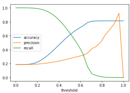
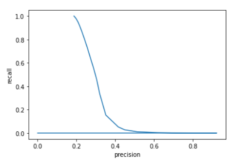
Unfortunately, you can’t have it both ways: increasing precision reduces recall, and vice versa. This is the so-called the precision/recall trade-off‰. In some contexts you will mainly care about precision, and in others you may really need high recall. Suppose you train a classifier to detect cancer, it is probably not too bad if your classifier has only 30% precision as long as it has 90% recall. Sure, the doctors can get false notifications, but almost all patients with cancer will be detected.

Finetune your model

At this point, if you are not satisfied with the performance of your model, you should go back and tune the model’s hyperparameters, for example the number of layers, the number of neurons per layer, the types of activation functions for each hidden layer, the number of training epochs.

Number of Hidden Layers and neurons

For many problems, you can just begin with a single hidden layer and you will get reasonable results. It has been shown that a multi-layer perceptron with only one or two hidden layers can model even the most complex problems provided that it has enough neurons. Of course, then the questions of how many neurons is enough comes into picture. Among some empirically derived rules of thumb, the most commonly relied on is ‘the optimal size of the hidden layer is usually between the size of the input and size of the output layers’. Have a look at this old post for further explanation. Unfortunately, from what I have read so far in books and machine learning communities, finding the perfect amount of neurons seems still somewhat a dark art. Just like for the number of layers, you can try increasing the number of neurons gradually until the network starts overfitting.

Activation function and optimizers

About the choice of activation function, in general, the rectified activation function will be a good default for all hidden layers. For the output layer, it really depends on your output value. Other options include choosing a better optimizer. This article provides some more insights about what you can do to fine-tune your model.

This concludes the basic introduction to artificial neural networks and their implementation with Tensor flow. I hope it is helpful. For more practice, I recommend practicing with different datasets and experimenting different parameters to see what impacts they have on your model performances.