Photo from Kasia Kulma on Slideshare

Despite a booming adoption of machine learning in making critical decisions, many machine learning models remain black boxes. Here trust and ethical challenges of using machine learning in making decisions come into the picture. Because the real-world consequences of wrong prediction can be expensive. In 2017, a lawsuit was filed against three US-based companies responsible for designing and developing an automated computer system which was used by Michigan government unemployment agency and made 20,000 false fraud accusations. A good boss will also question his data team why the company should be making these critical business decisions. In order not to blindly trust machine learning models, the need for understanding model’s behaviors, the decisions it makes, and any associated potential pitfalls is high on the agenda.

Model interpretability — Post hoc explanation technique

A commonly accepted phenomenon in data science community and literature (Johansson, Ulf, et al., 2011; Choi, Edward, et al., 2016, etc.) is that there is a trade-off between model accuracy and interpretability. At times
when you have a very large potentially complicated dataset, the use of complex models such as deep neural nets and random forests often achieve higher performance, but lower interpretability. In contrast, simpler models, such as linear or logistic regression just to name a few, often offer lower performance but higher interpretability. This is where post hoc explanation techniques emerge and become a game changer in machine learning literature.

Traditional statistical methods use a hypothesis-driven approach, which means that we construct the assumptions and verify hypotheses by training the models. Post hoc techniques, on the contrary, are set-up techniques which are applied “after the event”- after model training. So the idea people come up with is to first build complex models for making decisions and then explain them using simpler models. In other words, constructing complex model first and assumptions will come later. Some examples of post hoc explanation techniques include LIME, SHAP, Anchor, MUSE amongst others. My point of discussion in this article will be explaining what LIME is and how it works using a step-by-step guide with Python codes as well as the good and the ugly associated with LIME.

So what the heck is LIME and how does it work?

LIME is the abbreviation for Local Interpretable Model-agnostic Explanations. In essence, LIME is Model-agnostic, meaning that it can be applied to ANY models based on the assumption that every complex model is a black-box. By interpretable manner, it implies that LIME will be able to explain how the model behaves, which features it picks up and what kinds of interactions between them take place to drive the predictions. Last but certainly not least, LIME is observation specific, meaning that it tries to understand features that influence the black-box model around a single instance of interest. The rationale behind LIME is that as global model interpretability is very difficult to achieve in reality, it is far simpler to approximate a black-box model by a simple model locally.

In practice, the decision boundary of a black-box model can look very complex. In the figure below, the decision boundary of a black-box model is represented by the blue-pink background, which seems too complex to be accurately approximated by a linear model.

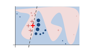Figure 1. Decision boundary of blackbox model. Source

However, studies (Baehrens, David, et al. (2010), Laugel et al., 2018 etc.) have shown that when you zoom in and look at a small enough neighborhood (bear with me, I will discuss what it means a meaningful neighborhood in the next session), no matter how complex the model is at a global level, the decision boundary at a local neighborhood can be a much more simpler, can in fact be even linear. For instance, the probability of someone having a cancer may be nonlinearly dependent on his age. But if you are looking at only a small group of people who are more than 70 so to say, there is a likelihood that for that subset of the population, the risk of having cancer is linearly correlated with increase in age.

That being said, what LIME does is to go on a very local level and get to a point where it becomes so local that a linear model is powerful enough to explain the behavior of the original black-box model at the local level and it will be highly accurate on that locality (in the neighborhood of the observation we want to explain). In the example (Figure 1), the bold red cross is the instance being explained. LIME will generate new instances by sampling a neighborhood around this selected instance, applying the original black-box model on that neighborhood to generate the corresponding predictions, and weighting those generated instances by their distances to the instance being explained.

In this obtained dataset (which includes the generated instances, the corresponding predictions and the weights), LIME trains an interpretable model (e.g weighted linear model, decision trees) which captures the behaviors of the complex model in that neighborhood. The coefficients of that local linear model will serve as the explanators and tell us which features drive the prediction to one way or the other. In Figure 1, the dashed line is the behaviour of the black-box model in a specific locality which can be explained by a linear model and the explanation is considered faithful in that locality.

Full recipe for LIME with a step-by-step guide (and Python codes)

import pandas as pd
import numpy as np
import matplotlib.pyplot as plt
from sklearn.ensemble import RandomForestClassifier
from sklearn.preprocessing import StandardScaler
import seaborn as sns

Part 1. Loading the data and training a Random Forest Model.

LIME can be applied to all types of data. The example developed in this article will limit to the analysis of tabular data. I use this data set of loan default on Hackereath. You can find a complete notebook on my GitHub. Since it was a quiet large dataset, I only make use of the trainingset as my full dataset for this example. Basically, I have a loan default dataset with the size of more than 500.000 observations and among features in that data set, I picked up 3 features (loan amount, annual income of borrowers and member_ID) which have the highest correlation with the target variable (default or non-default). You can find a summary of data used and follow the steps taken with the codes provided below.

#About the data
#Loan_status: Current status of the loan 0: default, 1: non-default #annual_inc: The reported annual income provided by the borrower
#loan_amnt: The listed amount of the loan applied for by the borrower.
#member_id: A unique assigned ID for customers.

#Loading dataset

df = pd.read_csv(“credit_default.csv”)#Plotting and doing some data

# Exploratory data analysis

ax1=df[‘annual_inc’].plot.hist()
ax1.set_xlabel(‘annual_inc’)
df.boxplot(column=[‘annual_inc’, ‘funded_amnt’,‘member_id’])

#Removing outliers for annual_income

Q1 = df[‘annual_inc’].quantile(0.25)
Q3 = df[‘annual_inc’].quantile(0.75)
IQR = Q3 - Q1
print(IQR)
df_outliers = df[(df[‘annual_inc’] < (Q1 - 1.5 * IQR)) | (df[‘annual_inc’] > (Q3 + 1.5 * IQR)) ]
df_clean = df[(df[‘annual_inc’] > (Q1 - 1.5 * IQR)) & (df[‘annual_inc’] < (Q3 + 1.5 * IQR)) ]

#Correlation matrix

sns.heatmap(data = df_clean.corr(),annot=True, linewidths=1.5, fmt=’.1g’,cmap=plt.cm.Reds)

# Picking up features for the model
features = [‘member_id’, ‘annual_inc’, ‘funded_amnt’]
tmp=df_clean[features]

#Standardization

X = StandardScaler().fit_transform(tmp)

#Training the model

from sklearn.model_selection import train_test_split
X_train,X_test,y_train,y_test=train_test_split(X,y,test_size = 0.33)
X_train.shape[0] == y_train.shape[0]from sklearn.ensemble import RandomForestClassifier
Model = RandomForestClassifier()

#Predicting using the test set and get accuracy, recall and precision score

Model.fit(X_train, y_train)y_predicted = Model.predict(X_test)
metrics.accuracy_score(y_test, y_predicted)
tn, fp, fn, tp = metrics.confusion_matrix(y_test,y_predicted).ravel()
recall = tp/(tp+fn)
precision = tp/(tp+fp)

print(“accuracy = {acc:0.3f},\nrecall = {recal:0.3f},\nprecision = {precision:0.3f}".format( acc=accuracy, recal=recall,precision=precision))

After training a Randome Forest model, I have an accuracy of 0.80 and a precision score of 0.61 and recall score of 0.44. Well, let’s move on with LIME explanation.

Part 2. LIME Explanation

Step 1. Select in your original dataset the instance of interest (Xi) for which you want to have an explanation for the black-box model.

Xi = np.array([ -0.71247975, -0.04996247, -1.02083371])

Given the fact that I have standardized the data in the previous step where I train the Random Forest model, here I will simply generate new instances (in the neighborhood of the instance being explained — Xi) by sampling from the normal distribution around Xi and standard deviation taken from the explanatory variables in training dataset.

num =750 # number of perturbations generated
sigma = 1 # Standard deviation
X_perturb = np.random.normal(Xi,sigma,size=(num,Xi.shape[0]))

If you have not standardized the data, LIME will internally do it for you. It should be noted that by default (have a look at LIME’s implementation in Python), LIME samples are taken from the mean of features data, which represents a global explanation. However, you can choose to sample data around the neighborhood of the instance of interest which is a more local-driven explanation. In this case, as mentioned, I choose to sample around the selected instance (Xi). If you sample around the mean of features, you might generate instanes which are far away from the instance for which you want an explanation. This is problematic because the explanation you get on your generated dataset can potentially differ from that of the instance being explained.

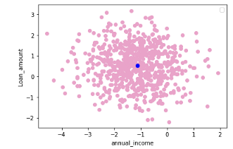
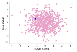Figure 2. Sampling around the instance being explained (in blue) (left) and sampling around the mean of feature data (right) — Visualization by author

Step 3. Make the prediction on that perturbed instances using the complex original black-box model

y_perturb = Model.predict(X_perturb)

Step 4.

Weight the generated samples according to their distances to the instance we want to explain. The weights are determined by a kernel function which takes euclidean distances and kernel width as input and outputs importance score (weight) for each generated instance.

distances = np.sum((Xi - X_perturb)**2,axis=1)#euclidean distance
kernel_width = 0.9 # I select a kernel width myself. By default in LIME, kernel width = 0.75 * sqrt(number of features)
weights = np.sqrt(np.exp(-(distances**2)/(kernel_width**2))) #Kernel function

LIME uses Euclidean distance as a similarity measure between the generated instances and the instance being explained. Does this figure below remind you of Pythagorean Theorem in Math class?

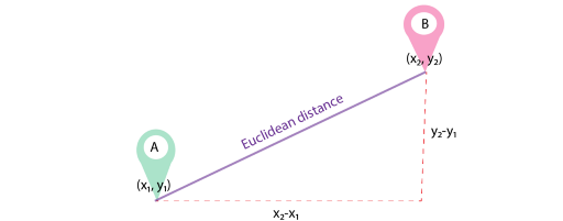
For n-dimensional data, the formula for Euclidean distance is as following:

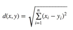
With regard to kernel width, By default, LIME’s implementation uses an exponential kernel where kernel width is set equal to 0.75 times the square root of the number of features (N) in the training dataset. You might wonder where this sqrt(N) comes from. Now suppose that vector σ = [σ1, σ2, σ3] are the standard deviations of vector features X [X1, X2, X3 ]. The sqrt(N) is the root mean square distance between the instance being explained and a generated instance. If we have a single feature and we generate a new instance, drawn from a normal distribution, the root mean square distance you expect will be equal to sigma (standard deviation). More formally, this distance is given by the root-mean-squared deviation. For N features that are statistically independent, and each drawn from a normal distribution, the mean-squares can be added equally and therefore the root-mean-squared deviation will be sqrt(N). or in formulas:

Step 5.

Train an interpretable local model (in this case, linear model) using the generated instances (X_perturb), corresponding predictions of the black-box model on the generated instances (y_perturb) and the weights (in step 4) to derive coefficients which serves as the explanation for the behaviors of black-box model at that locality. The coefficients of the local (linear) model will tell you which features drive the prediction of the black-box model to one way or the other.

from sklearn.linear_model import LinearRegression
local_model = LinearRegression()
local_model.fit(X_perturb, y_perturb, sample_weight=weights)
y_linmodel = local_model.predict(X_perturb)
local_model.coef_

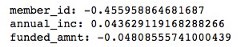Coefficients of local linear model — Calculation by author

The coefficients of the local models suggested that an increase in the funded amount (loan amount) drives the prediction towards default class (y = 0) meanwhile an increase in annual income will push prediction to non-defaul class (y =1). Figure 3 illustrates the 3-D decision boundary of the local model.

Figure 3. Plotting a 3D decision boundary of the local model. Visualization by author.

What is a meaningful neighbourhood?

As on every other case, the devil is in the detail. Achieving a meaningful locality is far from easy. A purposeful neighborhood needs to be small enough to achieve the local linearity. Plus, using a large neighborhood comes with the risk of producing a local model that produces an explanation which is not locally faithful. The reason being that when you create a large neighborhood, you run the risk of having instances which are far away and hence different from the instance for which you want an explanation. This would mean that the explanation of the black-box model on those far-away instances may differ from that of the selected instance and your explanation is biased towards a global level. Meanwhile, a too small neighborhood implies assigning high weight only to very close-by instances, indicating that you face the threat of under-sampling and the coefficients of the local model will be unstable around the surrounding neighborhood.

If you remember in step 4 (if not, please come back), the weights are determined by the so-called kernel width. Here things become tricky as the kernel width determines how large or small the neighborhood is. A small kernel width means that you assign more weight to the generated instances close by the instance whose prediction is being explained. Meanwhile, a large kernel width implies no matter how close/far the perturbed instances are from the original instance, they will still have certain influence on the local model. In figure 4, the size of the circles represent the weight.

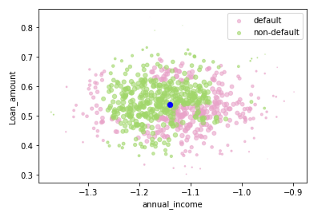
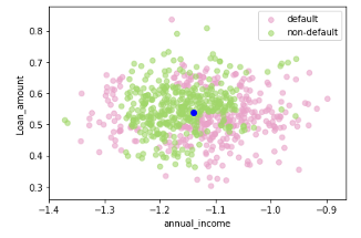Figure 4. Selecting a small kernel width (left) and large kernel width (right) — Visualization by Author

To see the impact of kernel width on the local explanation, in the figure 5, I illustrate how changes in kernel width will lead to changes in the coefficients of the local model. The default value for kernel width in LIME (0.75 times the square root of the number of features) is presented by the dotted line. Apparently, a kernel size with the value of 0.5 would be good to explain the behaviours of the blackbox model at that locality as going up from this threshold , local coefficients achieve stability. However, if we decreased the kernel width to 0.3 or lower, all three coefficients of the localmodel drastically change, indicating that from the threshold of 0.3, a decrease in the kernel size deteriorates the coefficient stability.

widths = np.linspace(0.01, sigma*np.sqrt(3), 1000)
alist = []
blist = []
clist = []
sigma = 1
for width in widths:
X_perturb, y_perturb, weights = make_perturbations(Xi, sigma=sigma, num=num_perturb, kernel_width = width, seed=8 )
a,c = get_local_coeffs(X_perturb, y_perturb, weights)
alist.append(a[0])
blist.append(a[1])
clist.append(a[2])
miny, maxy = np.min([alist,blist,clist]), np.max([alist,blist,clist])
plt.figure()
plt.plot(widths, alist, label = “coef1”, c = ‘yellow’)
plt.plot(widths, blist, label = “coef2”, c = ‘purple’)
plt.plot(widths, clist, label = “coef3”, c = ‘green’)
plt.plot([0.75*sigma*np.sqrt(3), 0.75*sigma*np.sqrt(3)], [miny, maxy], c='black’, ls=’:')
plt.ylim([miny,maxy])
plt.xlabel(“Kernel width”)
plt.ylabel(“Regression coefficient”)plt.legend()
plt.show()

Figure 5. Local_model coefficients for different kernel widths — Ilustration by author

To further confirm, I demonstrated the means and the confidence intervals of the coefficients for 100 different models with different kernel widths for the 3 features in my black-box model. The three solid lines (purple, blue and orange) represent the corresponding averaged coefficients of 100 different models. The shaded (purple, blue and orange) areas indicate 95% confidence intervals for each feature. As observed, the mean coefficients become less dispersed (represented by a smaller CI) with kernel widths larger than 0.3. At the same time, a kernel width smaller than 0.3 will lead to an instability in the coefficients for all features. Apparently, there is a trade-off between coefficients stability and kernel width (as a measure of locality level). In essence, to identify an optimal neighborhood, you aim to achieve the minimum kernel width where the coefficients of the linear models remain stable. This issue has been throughly analyzed and discussed by Alvarez-Melis, D., & Jaakkola, T. S. (2018) and Thomas, A. et al., (2020), you can have a look for further understanding.

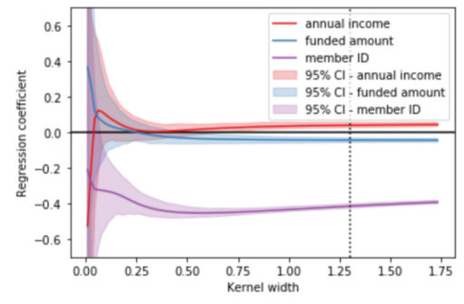Figure 6. Coefficients of 100 different local models for different kernel widths — Visualization by author

Beauty and the beast

So do I need LIME when I have high accuracy model? The problem is that, without knowing which symptoms the model picks to make the decisions, you do not know whether the model can give you the right answer for wrong reasons. As LIME is capable of finding local models, from its explanation, you can communicate to the domain experts and ask if that makes any sense. As such, LIME can aslo provide insights on how and why the black box model makes wrong predictions.

Can I trust in LIME? A couple of thoughts: First, LIME explanation is unstable because it depends on the number of fake instances you generate and the kernel width you select as discussed aboved. In some scenarios, you can completely change the direction of the explanation by changing the kernel width (as illustrated by the changes in coefficients in the figure 5,6).

Secondly, LIME is a post hoc technique based on assumption that things will have the linear relationship at local level. This is a very big assumption. At times when your black-box model is extremely complex and the model is simply not locally linear, a local explanation using linear model would not be good enough. That being said, we have to be very careful when a model is overly complex and adjust the kernel width accordingly. I highly doubt that LIME can be used to explain ANY complex models.

In a nutshell, LIME would be able to give a good local explanation — provided that a right neighborhood and the local linearity are achieved. But LIME should at the same time be used with great care due to potential pitfalls mentioned aboved.

Thank you for reading. I hope this helps with learning.

Originally published on Towards Data Science

References

[1] Alvarez-Melis, D., & Jaakkola, T. S. (2018). On the robustness of interpretability methods. arXiv preprint arXiv:1806.08049.9

[2] Baehrens, D., Schroeter, T., Harmeling, S., Kawanabe, M., Hansen, K., & MÞller, K. R. (2010). How to explain individual classification decisions. Journal of Machine Learning Research, 11(Jun), 1803–1831.

[3] Molnar, C. (2019). Interpretable machine learning. Lulu. com.

[4] Ribeiro, M. T., Singh, S., & Guestrin, C. (2016, August). “ Why should i trust you?” Explaining the predictions of any classifier. In Proceedings of the 22nd ACM SIGKDD international conference on knowledge discovery and data mining (pp. 1135–1144).

[5] Thomas, A. et al., Limitations of Interpretable Machine Learning Methods (2020)

[6] Medium blog on LIME by Lar

[7] Interpretable Machine Learning Using LIME Framework — Kasia Kulma (PhD), Data Scientist, Aviva — H2O.ai

Acknowledgement

Thanks Robert for discussions and helping me out with a nicely 3D plotting.